6. Plotting the graph structure
GNA is equipped with a module, that dumps the graph structure to the graphviz format. The computational graphs are
therefore may be plotted with dot command. In order to be used, a python module pygraphviz should be installed.
The computational graph may be plotted with savegraph function provided within gna.graphviz module. See the
usage example in the following macro:
 1from load import ROOT as R
 2import gna.constructors as C
 3import numpy as np
 4
 5n, n1, n2 = 12, 3, 4
 6
 7points_list = [ C.Points(np.arange(i, i+n).reshape(n1, n2)) for i in range(5) ]
 8tfactor = C.Points(np.linspace(0.5, 2.0, n).reshape(n1, n2))
 9tsum = C.Sum([p.points.points for p in points_list])
10tprod = C.Product([tsum.sum.sum, tfactor.points.points])
11
12for i, p in enumerate(points_list):
13    p.points.setLabel('Sum input:\nP{:d}'.format(i))
14tfactor.points.setLabel('Scale S')
15tsum.sum.setLabel('Sum of matrices')
16tprod.product.setLabel('Scaled matrix')
17tprod.product.product.setLabel('result')
18
19tsum.print()
20print()
21
22tprod.print()
23print()
24
25print('The sum:')
26print(tsum.transformations[0].outputs[0].data())
27print()
28
29print('The scale:')
30print(tfactor.transformations[0].outputs[0].data())
31print()
32
33print('The scaled sum:')
34print(tprod.transformations[0].outputs[0].data())
35print()
36
37from gna.graphviz import savegraph
38savegraph(tprod.transformations[0], tutorial_image_name('dot'), rankdir='TB')
39savegraph(tprod.transformations[0], tutorial_image_name('pdf'), rankdir='TB')
40savegraph(tprod.transformations[0], tutorial_image_name('png'), rankdir='TB')
Here we are using an example, similar to the one in the Sum tutorial. It implements the following formula:
Five matrices \(P\) are added together within Sum transformation. The result is then scaled by Product
transformation. The corresponding graph may be found below.
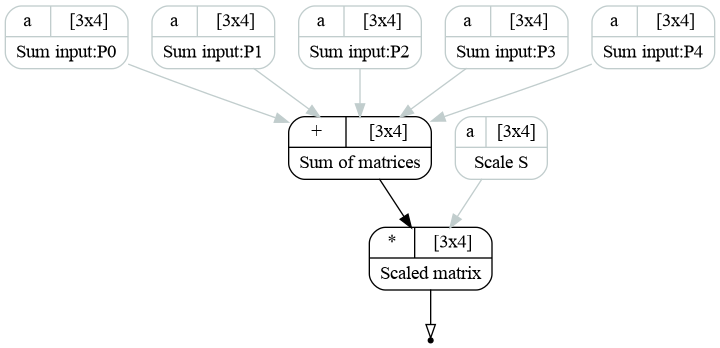
Example computational graph representing \(R_{ij} = S_{ij} \sum\limits_{k=1}^5 P_{ij}^k\).
Let us now look at how the graph is done. First of all proper labels should be introduced for nodes (transformations)
and, optionally, edges (inputs and outputs). This is done by the method setLabel(label). First of all it is applied
to each \(P_{ij}^k\):
for i, p in enumerate(points_list):
    p.points.setLabel('Sum input:\nP{:d}'.format(i))
The label may contain multiple lines. Here we used python format function (see pyformat.info for tutorial). Then we add labels for the sum, product and scale:
tfactor.points.setLabel('Scale S')
tsum.sum.setLabel('Sum of matrices')
tprod.product.setLabel('Scaled matrix')
Finally, we add label for the output:
tprod.product.product.setLabel('result')
Now, there is enough information to plot the graph with savegraph(transformation, filename) function:
savegraph(tprod.transformations[0], tutorial_image_name('dot'), rankdir='TB')
savegraph(tprod.transformations[0], tutorial_image_name('pdf'), rankdir='TB')
savegraph(tprod.transformations[0], tutorial_image_name('png'), rankdir='TB')
The first argument is transformation, output or list of transformations and outputs. The file format is either .dot, or an image format (.png, .pdf).
Optional argument rankdir defines the graph growth direction: ‘TB’ for top to bottom and ‘LR’ for left to right.
While the images are ready to use, the dot file may be opened with dot/xdot [1] applications:
xdot output/07_graphviz.dot
The .dot file is readable and may be edited by the user.