9.3.4. Replicating graphs
Now let us learn the second capability of the bundles: graph generation and replication. We will use the example of the energy resolution transformation. In short, the energy resolution transformation smears the input histogram bin by bin. Each bin is smeared with a Gaussian. A width is defined based on the bin center by a formula, that depends on three parameters: \(a\), \(b\) and \(c\).
The energy resolution object contains 2+ transformations: matrix transformation computes the smearing matrix based on the values of the parameters, at least one smear transformation smears the input histogram with smearing matrix.
We now will define a bundle which:
Defines the parameters for \(a\), \(b\) and \(c\).
If major index is specified, different parameters are defined for each iteration.
Minor indices are ignored.
Defines the energy resolution object for each major iteration.
The matrix transformation depends on the current parameters \(a\), \(b\) and \(c\). The bundle provides an input of the matrix transformation for each major iteration. The bin edges output should be connected to it.
New smear transformation is added for each minor iteration.
The bundle provides an input/output pair on each minor+major iteration.
Optional features:
Label formats.
Merge transformations. Do not create a new transformation for each minor index. Use the same transformation to process all the inputs. The procedure is explained here.
9.3.4.1. Energy resolution bundle
At first let us create a draft bundle detector_eres.
 1from gna.bundle import *
 2
 3class detector_eres_ex01(TransformationBundle):
 4    def __init__(self, *args, **kwargs):
 5        TransformationBundle.__init__(self, *args, **kwargs)
 6
 7    def build(self):
 8        self.objects = []
 9        for it_major in self.nidx_major:
10            vals = it_major.current_values(name=self.cfg.parameter)
11            names = [ '.'.join(vals+(name,)) for name in self.names ]
12
13            eres = C.EnergyResolution(names, ns=self.namespace)
14            self.objects.append(eres)
15
16            eres.print()
17
18            self.set_input('eres_matrix', it_major, eres.matrix.Edges, argument_number=0)
19
20            trans = eres.smear
21            for i, it_minor in enumerate(self.nidx_minor):
22                it = it_major + it_minor
23                eres.add_input()
24
25                self.set_input('eres', it, trans.inputs.back(), argument_number=0)
26                self.set_output('eres', it, trans.outputs.back())
27
28    def define_variables(self):
29        parname = self.cfg.parameter
30        parscfg = self.cfg.pars
31        self.names = None
32
33        for it_major in self.nidx_major:
34            major_values = it_major.current_values()
35            pars = parscfg[major_values]
36
37            if self.names is None:
38                self.names = tuple(pars.keys())
39            else:
40                assert self.names == tuple(pars.keys())
41
42            for i, (name, unc) in enumerate(pars.items()):
43                it=it_major
44
45                par = self.reqparameter(parname, it, cfg=unc, extra=name)
46
47
The method define_variables() is called to define th variables similarly to the tutorial on a bundle for parameters. The only difference is that for each major iteration there are three parameters to be defined. An extra check is done that the actual parameter names for each major iteration is the same.
Let us now look at the second method build() that creates a part of the computational graph.
 1        self.objects = []
 2        for it_major in self.nidx_major:
 3            vals = it_major.current_values(name=self.cfg.parameter)
 4            names = [ '.'.join(vals+(name,)) for name in self.names ]
 5
 6            eres = C.EnergyResolution(names, ns=self.namespace)
 7            self.objects.append(eres)
 8
 9            eres.print()
10
11            self.set_input('eres_matrix', it_major, eres.matrix.Edges, argument_number=0)
12
13            trans = eres.smear
14            for i, it_minor in enumerate(self.nidx_minor):
15                it = it_major + it_minor
16                eres.add_input()
17
18                self.set_input('eres', it, trans.inputs.back(), argument_number=0)
19                self.set_output('eres', it, trans.outputs.back())
20
We start from iterating over major indices combinations:
1        self.objects = []
2        for it_major in self.nidx_major:
3            vals = it_major.current_values(name=self.cfg.parameter)
4            names = [ '.'.join(vals+(name,)) for name in self.names ]
5
On each iteration we make a list of parameter names to be passed to the energy resolution constructor
1 self.objects.append(eres)
The namespace is passed to ensure that energy resolution refers to the correct parameters. Here is the contents of the EnergyResolution object:
[obj] EnergyResolution: 2 transformation(s), 3 variables
 0 [trans] matrix: 1 input(s), 1 output(s)
     0 [in]  Edges <- ...
     0 [out] FakeMatrix: invalid
 1 [trans] smear: 2 input(s), 1 output(s)
     0 [in]  FakeMatrix <- [out] FakeMatrix: invalid
     1 [in]  Ntrue <- ...
     0 [out] Nrec: invalid
As one can see and as described in EnergyResolution we need to bind a histogram that defines the bin edges to matrix.Edges and a histogram that will be smeared to the smear.Ntrue. Since the aim of the current bundle is not to bind the inputs and outputs, but rather to provide them to later use we declare the output with the following command:
1
The signature is set_input(‘name’, nidx, input, argument_number). The output will be located in the bundle.context.inputs.eres_matrix. The full path after bundle.context.inputs will be defined by the major index current format. Argument number will be added in the end of the path. It is used in case several inputs are used for the same name.
We then iterate over each minor index,
1            for i, it_minor in enumerate(self.nidx_minor):
2                it = it_major + it_minor
3                eres.add_input()
4
5                self.set_input('eres', it, trans.inputs.back(), argument_number=0)
6                self.set_output('eres', it, trans.outputs.back())
7
add a new input/output pair and declare the input/output pair with methods set_input() and set_output().
Now let us use the bundle in the following script:
 1import load
 2from gna.bundle import execute_bundle
 3from gna.configurator import NestedDict, uncertaindict, uncertain
 4from gna.env import env
 5from gna.bindings import common
 6from gna import constructors as C
 7import numpy as np
 8from matplotlib import pyplot as plt
 9
10cfg = NestedDict(
11    bundle = dict(
12        name='detector_eres',
13        version='ex01',
14        ),
15    parameter = 'eres',
16    pars = uncertaindict(
17        [
18         ('a', 0.01),
19         ('b', 0.09),
20         ('c', 0.03),
21         ],
22        mode='percent',
23        uncertainty = 30.0
24        ),
25)
26b = execute_bundle(cfg)
27env.globalns.printparameters(labels=True); print()
28
29#
30# Prepare inputs
31#
32emin, emax = 0.0, 12.0
33nbins = 240
34edges = np.linspace(emin, emax, nbins+1, dtype='d')
35data  = np.zeros(nbins, dtype='d')
36data[20]=1.0  # 1 MeV
37data[120]=1.0 # 6 MeV
38data[200]=1.0 # 10 MeV
39hist = C.Histogram(edges, data)
40hist.hist.setLabel('Input histogram')
41
42# Bind outputs
43#
44hist >> b.context.inputs.eres_matrix.values()
45hist >> b.context.inputs.eres.values()
46print( b.context )
47
48#
49# Plot
50#
51savegraph(hist, tutorial_image_name('png', suffix='graph'), rankdir='TB')
52
53fig = plt.figure()
54ax = plt.subplot(111, xlabel='E, MeV', ylabel='', title='Energy smearing')
55ax.minorticks_on()
56ax.grid()
57
58hist.hist.hist.plot_hist(label='Original histogram')
59b.context.outputs.eres.plot_hist(label='Smeared histogram')
60
61ax.legend(loc='upper right')
62
63savefig(tutorial_image_name('png'))
64plt.show()
The configuration and execution should be familiar to the use after tutorial on a bundle for parameters. The loaded parameters are the following:
Variables in namespace 'eres':
  a                    =       0.01 │        0.01±       0.003 [         30%] │
  b                    =       0.09 │        0.09±       0.027 [         30%] │
  c                    =       0.03 │        0.03±       0.009 [         30%] │
After executing the bundle let us make an input:
1emin, emax = 0.0, 12.0
2nbins = 240
3edges = np.linspace(emin, emax, nbins+1, dtype='d')
4data  = np.zeros(nbins, dtype='d')
5data[20]=1.0  # 1 MeV
6data[120]=1.0 # 6 MeV
7data[200]=1.0 # 10 MeV
8hist = C.Histogram(edges, data)
9hist.hist.setLabel('Input histogram')
Here we defined a histogram for energy between 0 and 12 MeV with three peaks: at 1 MeV, 6 MeV and 10 MeV. The histogram output is then bind to the inputs as follows:
1hist >> b.context.inputs.eres_matrix.values()
2hist >> b.context.inputs.eres.values()
3print( b.context )
The last line prints the contents of the context:
${
  inputs : ${
    eres_matrix : ${
      00 : [in]  Edges <- [out] hist: hist, 240 bins, edges 0.0->12.0, width 0.05,
    },
    eres : ${
      00 : [in]  Ntrue <- [out] hist: hist, 240 bins, edges 0.0->12.0, width 0.05,
    },
  },
  objects : ${},
  outputs : ${
    eres_matrix : [out] FakeMatrix: array 2d, shape 240x240, size 57600,
    eres : [out] Nrec: hist, 240 bins, edges 0.0->12.0, width 0.05,
  },
}
Context is a nested dictionary with declared inputs eres_matrix.00 and eres.00. The outputs contain outputs eres_matrix and eres. Just as it was declared in the bundle for the case with empty major iterator. When binding we have used .values() method that returns an iterator on all the values to avoid typing 00.
When empty multi-index is provided the resulting graph looks as follows:
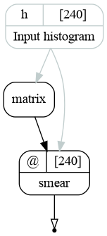
The resulting graph of the energy resolution bundle for the case of empty index.
It contains the matrix transformation, which is defined by the histogram binning. The matrix is then used to smear the histogram via smear transformation. As it is noted in the EnergyResolution, the input of the matrix is used only to define the matrix shape: it does not read the histogram and does not propagate the taint flag.
The example produces the following plot:
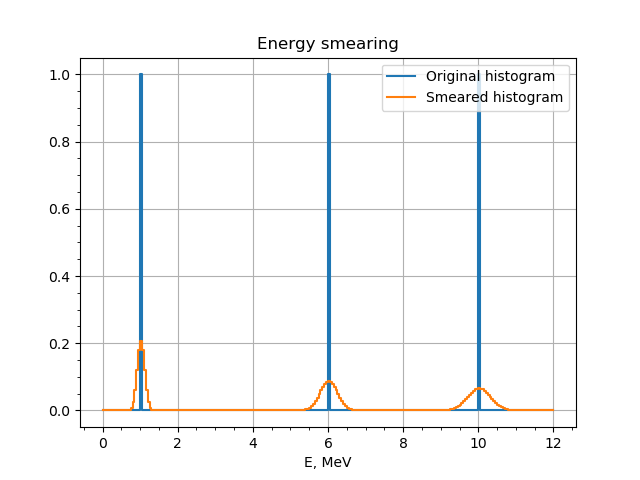
A histogram with bins at 1 MeV, 6 MeV and 10 MeV smeared with EnergyResolution bundle.
9.3.4.2. Energy resolution replicated
Before trying more complex example, we add some new features to the detector_eres bundle. We change the version mark to ex02 to keep both versions available. The updates include:
A method to label transformations and parameters based on the configuration.
Option split_transformations (true by default) which changes the graph topology.
The newer version is available in detector_eres_ex02.py.
Here is a script:
  1import load
  2from gna.bundle import execute_bundle
  3from gna.configurator import NestedDict, uncertaindict, uncertain
  4from gna import constructors as C
  5from gna.env import env
  6import numpy as np
  7from matplotlib import pyplot as plt
  8from gna.bindings import common
  9
 10cfg = NestedDict(
 11    bundle = dict(
 12        name='detector_eres',
 13        version='ex02',
 14        nidx=[ ('d', 'detector', ['D1', 'D2', 'D3']),
 15               ('z', 'zone', ['z1', 'z2'])],
 16        major=['z'],
 17        names=dict(
 18            eres_matrix='smearing_matrix',
 19            )
 20        ),
 21    parameter = 'eres',
 22    pars = uncertaindict(
 23        [
 24         ('z1.a', (0.0, 'fixed')),
 25         ('z1.b', (0.05, 30, 'percent')),
 26         ('z1.c', (0.0, 'fixed')),
 27         ('z2.a', (0.0, 'fixed')),
 28         ('z2.b', (0.10, 30, 'percent')),
 29         ('z2.c', (0.0, 'fixed')),
 30         ('z3.a', (0.0, 'fixed')),
 31         ('z3.b', (0.15, 30, 'percent')) ,
 32         ('z3.c', (0.0, 'fixed')),
 33         ]
 34        ),
 35    labels = dict(
 36        matrix    = 'Smearing\nmatrix\n{autoindex}',
 37        smear     = 'Energy\nresolution\n{autoindex}',
 38        parameter = '{description} (zone {autoindex})'
 39        ),
 40    split_transformations = True
 41)
 42b = execute_bundle(cfg)
 43env.globalns.printparameters(labels=True); print()
 44
 45#
 46# Prepare inputs
 47#
 48emin, emax = 0.0, 12.0
 49nbins = 240
 50edges = np.linspace(emin, emax, nbins+1, dtype='d')
 51data1  = np.zeros(nbins, dtype='d')
 52data1[20]=1.0  # 1 MeV
 53data1[120]=1.0 # 6 MeV
 54data1[200]=1.0 # 10 MeV
 55
 56data2  = np.zeros(nbins, dtype='d')
 57data2[40]=1.0  # 2 MeV
 58data2[140]=1.0 # 7 MeV
 59data2[220]=1.0 # 11 MeV
 60
 61data3  = np.zeros(nbins, dtype='d')
 62data3[60]=1.0  # 3 MeV
 63data3[160]=1.0 # 8 MeV
 64data3[239]=1.0 # 12 MeV
 65
 66hist1 = C.Histogram(edges, data1)
 67hist1.hist.setLabel('Input histogram 1')
 68
 69hist2 = C.Histogram(edges, data2)
 70hist2.hist.setLabel('Input histogram 2')
 71
 72hist3 = C.Histogram(edges, data3)
 73hist3.hist.setLabel('Input histogram 3')
 74
 75#
 76# Bind outputs
 77#
 78suffix = '' if cfg.split_transformations else 'merged_'
 79savegraph(b.context.outputs.smearing_matrix.values(), tutorial_image_name('png', suffix=suffix+'graph0'), rankdir='TB')
 80
 81hist1   >> b.context.inputs.smearing_matrix.values(nested=True)
 82hist1   >> b.context.inputs.eres.D1.values(nested=True)
 83hist2   >> b.context.inputs.eres.D2.values(nested=True)
 84hist3   >> b.context.inputs.eres.D3.values(nested=True)
 85print( b.context )
 86
 87savegraph(hist1, tutorial_image_name('png', suffix=suffix+'graph1'), rankdir='TB')
 88
 89#
 90# Plot
 91#
 92fig = plt.figure(figsize=(12,12))
 93
 94hists = [hist1, hist2, hist3]
 95for i, det in enumerate(['D1', 'D2', 'D3']):
 96    ax = plt.subplot(221+i, xlabel='E, MeV', ylabel='', title='Energy smearing in '+det)
 97    ax.minorticks_on()
 98    ax.grid()
 99
100    hists[i].hist.hist.plot_hist(label='Original histogram')
101    for i, out in enumerate(b.context.outputs.eres[det].values(nested=True)):
102        out.plot_hist(label='Smeared histogram (%i)'%i)
103
104    ax.legend(loc='upper right')
105
106savefig(tutorial_image_name('png'))
107plt.show()
Let us look at the configuration in more details. First of all we defined indices.
1        nidx=[ ('d', 'detector', ['D1', 'D2', 'D3']),
2               ('z', 'zone', ['z1', 'z2'])],
3        major=['z'],
We assume that there are three detectors D1, D2 and D3 with same energy resolution parameters. In the same time, each of the detectors has two zones z1 and z2 with own parameters. The zone index z is thus major while the detector index d is minor. The parameters configuration contains a value and uncertainty for each of the parameters \(a\), \(b\) and \(c\) for each of the zones.
 1    pars = uncertaindict(
 2        [
 3         ('z1.a', (0.0, 'fixed')),
 4         ('z1.b', (0.05, 30, 'percent')),
 5         ('z1.c', (0.0, 'fixed')),
 6         ('z2.a', (0.0, 'fixed')),
 7         ('z2.b', (0.10, 30, 'percent')),
 8         ('z2.c', (0.0, 'fixed')),
 9         ('z3.a', (0.0, 'fixed')),
10         ('z3.b', (0.15, 30, 'percent')) ,
11         ('z3.c', (0.0, 'fixed')),
12         ]
13        ),
One may see that there are parameters for more zones in the configuration, but only ones, defined by indices, will be read.
Also, the bundle normally defines input/output pairs for eres and eres_matrix. These names may be overridden via dictionary names in the bundle configuration:
1        names=dict(
2            eres_matrix='smearing_matrix',
3            )
Here we have defined a new name smearing_matrix for the eres_matrix. Name substitutions are realized by the GNA.
By using labels we now define the labels for matrix and smear transformations and for the parameters. The format strings include the field {autoindex} that will be substituted by the current iteration of the multi-index. There is also {description} field, that will be substituted by the parameter meaning. The labels are set by the detector_eres bundle of version ex02.
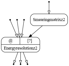
Executing the bundle we produce the following graph:
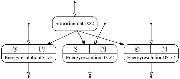
The resulting graph of the energy resolution bundle (version ex02). Inputs are open.
As one may see, there are two smearing matrices, one for each zone. The matrices are similar between the detectors.
The parameters are defined for each of the zones:
Variables in namespace 'eres.z1':
  a                    =          0 │                 [fixed]                 │ spatial/temporal resolution (zone z1)
  b                    =       0.05 │        0.05±       0.015 [         30%] │ photon statistics (zone z1)
  c                    =          0 │                 [fixed]                 │ dark noise (zone z1)
Variables in namespace 'eres.z2':
  a                    =          0 │                 [fixed]                 │ spatial/temporal resolution (zone z2)
  b                    =        0.1 │         0.1±        0.03 [         30%] │ photon statistics (zone z2)
  c                    =          0 │                 [fixed]                 │ dark noise (zone z2)
We now define input histograms in the same way as we done in the previous example with the only difference. There is now a separate histogram for each detector with the peaks in the different positions.
 1emin, emax = 0.0, 12.0
 2nbins = 240
 3edges = np.linspace(emin, emax, nbins+1, dtype='d')
 4data1  = np.zeros(nbins, dtype='d')
 5data1[20]=1.0  # 1 MeV
 6data1[120]=1.0 # 6 MeV
 7data1[200]=1.0 # 10 MeV
 8
 9data2  = np.zeros(nbins, dtype='d')
10data2[40]=1.0  # 2 MeV
11data2[140]=1.0 # 7 MeV
12data2[220]=1.0 # 11 MeV
13
14data3  = np.zeros(nbins, dtype='d')
15data3[60]=1.0  # 3 MeV
16data3[160]=1.0 # 8 MeV
17data3[239]=1.0 # 12 MeV
18
19hist1 = C.Histogram(edges, data1)
20hist1.hist.setLabel('Input histogram 1')
21
22hist2 = C.Histogram(edges, data2)
23hist2.hist.setLabel('Input histogram 2')
24
25hist3 = C.Histogram(edges, data3)
26hist3.hist.setLabel('Input histogram 3')
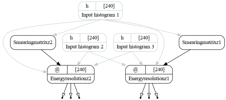
We bind the first histogram to the matrix input. Each histogram hist1, hist2 and hist3 is the binded to all the inputs of detectors D1, D2 and D3 respectively.
1hist1   >> b.context.inputs.smearing_matrix.values(nested=True)
2hist1   >> b.context.inputs.eres.D1.values(nested=True)
3hist2   >> b.context.inputs.eres.D2.values(nested=True)
4hist3   >> b.context.inputs.eres.D3.values(nested=True)
We have used nestsed=True key that returns all the values in all the nested dictionaries regardless of the structure. The full graph now looks as follows:
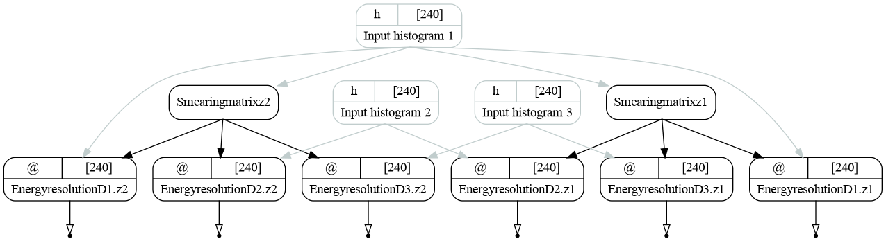
The resulting graph of the energy resolution bundle (version ex02). Inputs are bound.
And the result of the smearing plotted:
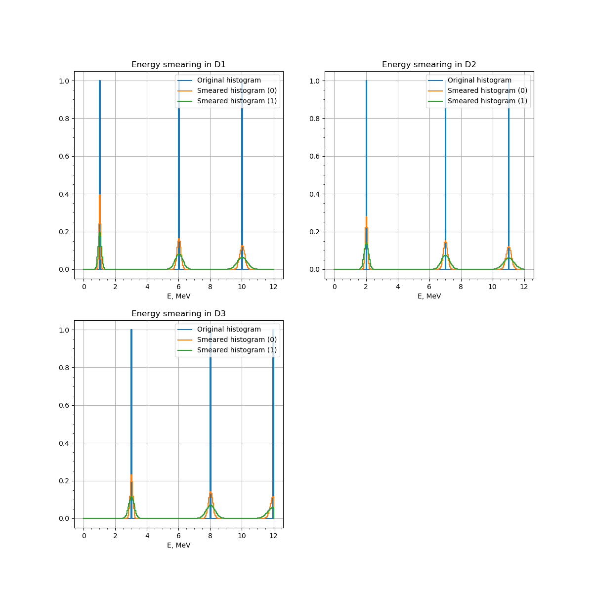
Three histograms (D1, D2 and D3) smeared with two smear matrices each (z1 and z2).
9.3.4.3. Energy resolution replicated (and merged)
The computational chain topology is discussed in tutorial Lazy evaluation and graph structure. The detector_eres bundle has parameter split_transformations, which is by default True. This means that each minor iteration produces an input in a new transformation: each input taintflag is propagated in separate. If split_transformations is set to False, all the inputs for the same major iteration are handled by the same transformation as shown in the following graph.
The resulting graph of the energy resolution bundle (version ex02) with split_transformations=False. Inputs are open.
When the histograms are bound to the inputs, the graph looks as follows:
The resulting graph of the energy resolution bundle (version ex02) with split_transformations=False. Inputs are bound.