8.3.1. Lazy evaluation and graph structure
8.3.1.1. Introduction
In this section we will take a closer look on taintflag propagation and on how the graph is evaluated. We will look at two examples. Each example defines integrals of two functions:
The functions depend on different parameters. The only difference between examples is that first one does integration with two distinct transformations while the second reuses a single transformation to integrate both functions. Examples are based on the code from tutorials 1d integration and More on 1d integration.
8.3.1.2. Example 1: separate transformations
The first example goes as follows:
  1import load
  2from gna.env import env
  3import gna.constructors as C
  4import numpy as np
  5from matplotlib import pyplot as plt
  6import matplotlib.gridspec as gridspec
  7from gna.bindings import common
  8import ROOT as R
  9
 10# Make a variable for global namespace
 11ns = env.globalns
 12
 13# Create a parameter in the global namespace
 14p1a = ns.defparameter('fcn1.a', central=1.0, free=True, label='weight 1')
 15p1b = ns.defparameter('fcn1.b', central=0.2, free=True, label='weight 2')
 16p1k = ns.defparameter('fcn1.k', central=8.0, free=True, label='argument scale')
 17
 18p2a = ns.defparameter('fcn2.a', central=0.5, free=True, label='weight 1')
 19p2b = ns.defparameter('fcn2.b', central=0.1, free=True, label='weight 2')
 20p2k = ns.defparameter('fcn2.k', central=16.0, free=True, label='argument scale')
 21
 22# Print the list of parameters
 23ns.printparameters(labels=True)
 24print()
 25
 26# Define binning and integration orders
 27nbins = 20
 28x_edges = np.linspace(-np.pi, np.pi, nbins+1, dtype='d')
 29x_widths = x_edges[1:]-x_edges[:-1]
 30x_width_ratio = x_widths/x_widths.min()
 31orders = 4
 32
 33# Initialize histogram
 34hist = C.Histogram(x_edges)
 35
 36# Initialize integrator
 37integrator = R.IntegratorGL(nbins, orders)
 38integrator.points.edges(hist.hist.hist)
 39int_points = integrator.points.x
 40
 41# Initialize sine and two cosines
 42sin_t = R.Sin(int_points)
 43cos1_arg = C.WeightedSum( ['fcn1.k'], [int_points] )
 44cos2_arg = C.WeightedSum( ['fcn2.k'], [int_points] )
 45
 46cos1_t = R.Cos(cos1_arg.sum.sum)
 47cos2_t = R.Cos(cos2_arg.sum.sum)
 48
 49# Initalizes both weighted sums
 50fcn1   = C.WeightedSum(['fcn1.a', 'fcn1.b'], [sin_t.sin.result, cos1_t.cos.result])
 51fcn2   = C.WeightedSum(['fcn2.a', 'fcn2.b'], [sin_t.sin.result, cos2_t.cos.result])
 52
 53# Create two debug transformations to check the execution
 54dbg1a = R.DebugTransformation('before int1', 1.0)
 55dbg2a = R.DebugTransformation('before int2', 1.0)
 56dbg1b = R.DebugTransformation('after int1', 1.0)
 57dbg2b = R.DebugTransformation('after int2', 1.0)
 58
 59# Connect inputs (debug 1)
 60print('Connect to inputs')
 61dbg1a.add_input(fcn1.sum.sum)
 62dbg2a.add_input(fcn2.sum.sum)
 63print()
 64
 65# Connect outputs (debug 1) to the integrators
 66print('Connect outputs')
 67int1 = integrator.transformations.back()
 68integrator.add_input(dbg1a.debug.target)
 69int2 = integrator.add_transformation()
 70integrator.add_input(dbg2a.debug.target)
 71print()
 72
 73# Connect inputs of debug transformations
 74print('Connect to inputs')
 75dbg1b.add_input(int1.hist)
 76dbg2b.add_input(int2.hist)
 77print()
 78
 79# Read outputs of debug transformations
 80print('Read data 1: 1st')
 81dbg1b.debug.target.data()
 82print()
 83
 84print('Read data 1: 2d')
 85dbg1b.debug.target.data()
 86print('    <no functions executed>')
 87print()
 88
 89print('Read data 2d 1st')
 90dbg2b.debug.target.data()
 91print()
 92
 93print('Read data 2d 2d')
 94dbg2b.debug.target.data()
 95print('    <no functions executed>')
 96print()
 97
 98# Change parameter k1 which affects only the first integrand
 99print('Change k1')
100p1k.set(9)
101
102# Read outputs of debug transformations
103print('Read data 1: 1st')
104dbg1b.debug.target.data()
105print()
106
107print('Read data 1: 2d')
108dbg1b.debug.target.data()
109print('    <no functions executed>')
110print()
111
112print('Read data 2d 1st')
113dbg2b.debug.target.data()
114print('    <no functions executed>')
115print()
116
117print('Read data 2d 2d')
118dbg2b.debug.target.data()
119print('    <no functions executed>')
120print()
121
122print('Done')
123
124integrator.print()
125print()
126
127print(dbg1b.debug.target.data().sum(), dbg2b.debug.target.data().sum())
128
129# # Label transformations
130hist.hist.setLabel('Input histogram\n(bins definition)')
131integrator.points.setLabel('Sampler\n(Gauss-Legendre)')
132sin_t.sin.setLabel('sin(x)')
133cos1_arg.sum.setLabel('k1*x')
134cos2_arg.sum.setLabel('k2*x')
135cos1_t.cos.setLabel('cos(k1*x)')
136cos2_t.cos.setLabel('cos(k2*x)')
137int1.setLabel('Integrator 1\n(convolution)')
138int2.setLabel('Integrator 2\n(convolution)')
139fcn1.sum.setLabel('a1*sin(x) + b1*cos(k1*x)')
140fcn2.sum.setLabel('a2*sin(x) + b2*cos(k2*x)')
141dbg1a.debug.setLabel('Debug 1\n(before integral 1)')
142dbg2a.debug.setLabel('Debug 2\n(before integral 2)')
143dbg1b.debug.setLabel('Debug 1\n(after integral 1)')
144dbg2b.debug.setLabel('Debug 2\n(after integral 2)')
145
146savegraph(int_points, tutorial_image_name('png', suffix='graph'), rankdir='TB')
147
148plt.show()
It produces the following graph.
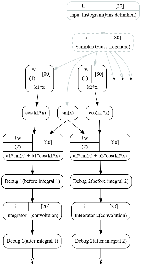
Computatinal graph used to compute integrals of functions (1). Each integration is handled by distinct integrator.
As before the procedure starts from the bins and integration points definition. The integration points then go to the transformation implementing \(sin(x)\) which is same for both functions. Cosines are computed in separate branches. The functions and integrations are then done in separate branches as well.
Note there are 4 debug transformations before and after each integration. Debug transformations print to the terminal, when the transformation their functions are executed. This will help us track the procedure of graph execution.
They are created with the following commands:
dbg1a = R.DebugTransformation('before int1', 1.0)
dbg2a = R.DebugTransformation('before int2', 1.0)
dbg1b = R.DebugTransformation('after int1', 1.0)
dbg2b = R.DebugTransformation('after int2', 1.0)
The first argument defines the name which will be printed to the output, the second argument is a delay \(D\). The transformation function will sleep for \(D\) seconds if executed. The debug transformation has the same number of outputs as the number of inputs. Its input is directly copied to the corresponding output.
The integrators are created with the following lines:
1int1 = integrator.transformations.back()
2integrator.add_input(dbg1a.debug.target)
3int2 = integrator.add_transformation()
4integrator.add_input(dbg2a.debug.target)
At first we simply save the first integrator for later use (labels and binding). Then we bind the output of first debug transformation to the input of the integrator via add_input(output) method. The second instance of the integrator is created with add_transformation() method. The second integrand is again added with the add_input(output) method.
The status of the integrator object confirms that we have created two integrator instances (hist and hist_02) and each of them has an input bound to the output of the function (through the debug transformation).
[obj] IntegratorGL: 3 transformation(s), 0 variables
 0 [trans] points: 1 input(s), 2 output(s)
     0 [in]  edges <- [out] hist: hist,  20 bins, edges -3.14159265359->3.14159265359, width 0.314159265359
     0 [out] x: array 1d, shape 80, size  80
     1 [out] xedges: hist,  21 bins, edges -3.14159265359->3.14159265359, width 0.314159265359
 1 [trans] hist: 1 input(s), 1 output(s)
     0 [in]  f <- [out] target: array 1d, shape 80, size  80
     0 [out] hist: hist,  20 bins, edges -3.14159265359->3.14159265359, width 0.314159265359
 2 [trans] hist_02: 1 input(s), 1 output(s)
     0 [in]  f <- [out] target: array 1d, shape 80, size  80
     0 [out] hist: hist,  20 bins, edges -3.14159265359->3.14159265359, width 0.314159265359
After the computational graph is constructed let us access the output of each last transformation twice:
dbg1b.debug.target.data()
dbg1b.debug.target.data()
dbg2b.debug.target.data()
dbg2b.debug.target.data()
Here is the corresponding terminal output:
Read data 1: 1st
    debug: executing transformation function (#1) [before int1]
    debug: sleep for 1 second(s)... done. [before int1]
    debug: executing transformation function (#1) [after int1]
    debug: sleep for 1 second(s)... done. [after int1]

Read data 1: 2d
    <no functions executed>

Read data 2d 1st
    debug: executing transformation function (#1) [before int2]
    debug: sleep for 1 second(s)... done. [before int2]
    debug: executing transformation function (#1) [after int2]
    debug: sleep for 1 second(s)... done. [after int2]

Read data 2d 2d
    <no functions executed>
As we read the output of the first branch, it triggers the execution of the transformations needed for this branch only. As one can see, no debug output associated with second integral happens after first data access. On the second data access to the same branch no execution happens: the transformation simply returns the cached result.
Only when the output of the second branch is read, the remaining transformations are triggered. Again, on the second access no execution happens.
Next we change the value of \(k_1\) coefficient, that affects the branch 1 via cosine:
p1k.set(9)
and repeat the procedure of reading data from both branches twice. Here is the result:
Read data 1: 1st
    debug: executing transformation function (#2) [before int1]
    debug: sleep for 1 second(s)... done. [before int1]
    debug: executing transformation function (#2) [after int1]
    debug: sleep for 1 second(s)... done. [after int1]

Read data 1: 2d
    <no functions executed>

Read data 2d 1st
    <no functions executed>

Read data 2d 2d
    <no functions executed>
As one can see, only the first branch integral was triggered. The second branch returned the cached value as it is not affected by \(k_1\).
Note
The actual execution happens only when data is read, but not by the change of the value of \(k_1\).
8.3.1.3. Example 2: merged transformations
The code for the second example is mostly identical to the previous one so we only highlight the part that is different:
1int1 = integrator.transformations.back()
2integrator.add_input(dbg1a.debug.target)
3integrator.add_input(dbg2a.debug.target)
These lines represent the binding of the integrator inputs. As we do not create the second integration here, both add_input(output) calls bind the outputs to the same integrator.
[obj] IntegratorGL: 2 transformation(s), 0 variables
 0 [trans] points: 1 input(s), 2 output(s)
     0 [in]  edges <- [out] hist: hist,  20 bins, edges -3.14159265359->3.14159265359, width 0.314159265359
     0 [out] x: array 1d, shape 80, size  80
     1 [out] xedges: hist,  21 bins, edges -3.14159265359->3.14159265359, width 0.314159265359
 1 [trans] hist: 2 input(s), 2 output(s)
     0 [in]  f <- [out] target: array 1d, shape 80, size  80
     1 [in]  f_02 <- [out] target: array 1d, shape 80, size  80
     0 [out] hist: hist,  20 bins, edges -3.14159265359->3.14159265359, width 0.314159265359
     1 [out] hist_02: hist,  20 bins, edges -3.14159265359->3.14159265359, width 0.314159265359
The graph looks as follows [1].
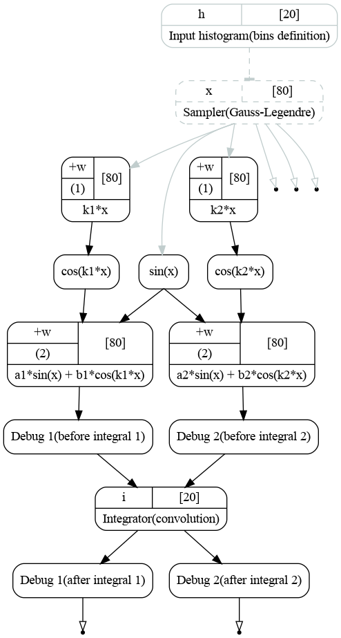
Computatinal graph used to compute integrals of functions (1). Both integrations are handled by a single transformation.
We now repeat the procedure of accessing the data outputs.
Read data 1: 1st
    debug: executing transformation function (#1) [before int1]
    debug: sleep for 1 second(s)... done. [before int1]
    debug: executing transformation function (#1) [before int2]
    debug: sleep for 1 second(s)... done. [before int2]
    debug: executing transformation function (#1) [after int1]
    debug: sleep for 1 second(s)... done. [after int1]

Read data 1: 2d
    <no functions executed>

Read data 2d 1st
    debug: executing transformation function (#1) [after int2]
    debug: sleep for 1 second(s)... done. [after int2]

Read data 2d 2d
    <no functions executed>
As one can see, since the integrator is reading all its inputs, both branches before the integrator are triggered on the first data access. The last debug in the second branch is not executed since it is not required for the first branch. It is then executed, when the second branch is accessed.
Absolutely the same thing happens after we change the value of the coefficient \(k_1\).
Read data 1: 1st
    debug: executing transformation function (#2) [before int1]
    debug: sleep for 1 second(s)... done. [before int1]
    debug: executing transformation function (#2) [after int1]
    debug: sleep for 1 second(s)... done. [after int1]

Read data 1: 2d
    <no functions executed>

Read data 2d 1st
    debug: executing transformation function (#2) [after int2]
    debug: sleep for 1 second(s)... done. [after int2]

Read data 2d 2d
    <no functions executed>
The integrator execution is triggered by the data access after the \(k_1\) is changed. Integrator then will integrate the branch 2 regardless of was it tainted or not.
8.3.1.4. Conclusions
The two presented graph structures produce the same numerical result but do differ in terms of execution order and efficiency:
Having separate transformations for each operation provides very good granularity. Such a cases will be efficient when there are a lot of parameters and the parameters are changed one at a time making a good use of caching and lazy evaluation.
Merging a lot of transformations together is potentially efficient in cases, when the overhead of function execution itself is more important then the impact of granularity and the array sizes, i.e. for usage on GPUs. In this case it may happen to be more efficient to compute a lot of branches in the same call than taking care on which of them are required to be recalculated.
As soon as we are planning to provide the GPU support we will take care on changing the graph structure. Most of the objects will be provided with methods similar add_transformation() and add_input() and ability to switch between one-transformation/multiple-inputs and single-input/multiple-transformations strategies.