8.2.1. 1d interpolation
In this example we will review another object defined by two transformations. InterpExpo implements exponential interpolation. For a function defined as set of points \(y_j(x_j)\), the interpolation function reads as follows:
The coefficients \(b_j\) are chosen so that the function was continuous. The example goes as follows.
  1from load import ROOT as R
  2import gna.constructors as C
  3import numpy as np
  4from matplotlib import pyplot as plt
  5from gna.bindings import common
  6from gna.env import env
  7
  8# Initialize segment edges and sampling points
  9xmin, xmax = 1.0, 11.0
 10nsegments = 10
 11npoints   = 100
 12edges = C.Points(np.linspace(xmin, xmax, nsegments+1, dtype='d'), labels='Coarse x')
 13edges_data = edges.single().data()
 14
 15points = np.linspace(xmin, xmax, npoints+1, dtype='d')
 16np.random.shuffle(points)
 17points   = C.Points(points, labels='Fine x\n(shuffled)')
 18# Note: sampling points are shuffled
 19
 20# Initialize raw function
 21y0 = np.exp(1/edges.single().data()**0.5)
 22# Make it saw-like by scaling all odd and even points to different sides
 23y0[::2]*=1.4
 24y0[1::2]*=0.7
 25y0 = C.Points(y0, labels='Coarse y\n(not scaled)')
 26
 27# Define two sets of scales to correct each value of y0
 28pars1 = env.globalns('pars1')
 29pars2 = env.globalns('pars2')
 30for ns in (pars1, pars2):
 31    for i in range(nsegments+1):
 32        ns.defparameter('par_{:02d}'.format(i), central=1, free=True, label='Scale for x_{}={}'.format(i, edges_data[i]))
 33
 34# Initialize transformations for scales
 35with pars1:
 36    varray1=C.VarArray(list(pars1.keys()), labels='Scales 1\n(p1)')
 37
 38with pars2:
 39    varray2=C.VarArray(list(pars2.keys()), labels='Scales 2\n(p2)')
 40
 41# Make two products: y0 scaled by varray1 and varray2
 42y1 = C.Product([varray1.single(), y0.single()], labels='p1*y')
 43y2 = C.Product([varray2.single(), y0.single()], labels='p2*y')
 44
 45# Initialize interpolator
 46manual = False
 47labels=('Segment index\n(fine x in coarse x)', 'Interpolator')
 48if manual:
 49    # Bind transformations manually
 50    interpolator = R.InterpExpo(labels=labels)
 51
 52    edges  >> (interpolator.insegment.edges, interpolator.interp.x)
 53    points >> (interpolator.insegment.points, interpolator.interp.newx)
 54    interpolator.insegment.insegment >> interpolator.interp.insegment
 55    interpolator.insegment.widths    >> interpolator.interp.widths
 56    y1 >> interpolator.interp.y
 57    y2 >> interpolator.add_input()
 58
 59    interp1, interp2 = interpolator.interp.outputs.values()
 60else:
 61    # Bind transformations automatically
 62    interpolator = R.InterpExpo(edges, points, labels=labels)
 63    interp1 = interpolator.add_input(y1)
 64    interp2 = interpolator.add_input(y2)
 65
 66# Print the interpolator status
 67interpolator.print()
 68
 69# Change each second parameter for second curve
 70for par in list(pars2.values())[1::2]:
 71    par.set(2.0)
 72
 73# Print parameters
 74env.globalns.printparameters(labels=True)
 75
 76# Plot graphs
 77fig = plt.figure()
 78ax = plt.subplot(111, xlabel='x', ylabel='y', title='Interpolation')
 79ax.minorticks_on()
 80
 81y0.points.points.plot_vs(edges.single(), '--', label='Original function')
 82interp1.plot_vs(points.single(), 's', label='Interpolation (scale 1)', markerfacecolor='none')
 83interp2.plot_vs(points.single(), '^', label='Interpolation (scale 2)', markerfacecolor='none')
 84
 85for par in list(pars1.values())[::2]:
 86    par.set(0.50)
 87
 88interp1.plot_vs(points.single(), 'v', label='Interpolation (scale 1, modified)', markerfacecolor='none')
 89
 90ax.autoscale(enable=True, axis='y')
 91ymin, ymax = ax.get_ylim()
 92ax.vlines(edges_data, ymin, ymax, linestyle='--', label='Segment edges', alpha=0.5, linewidth=0.5)
 93
 94ax.legend(loc='upper right')
 95
 96# Save figure and graph as images
 97savefig(tutorial_image_name('png'))
 98savegraph(points, tutorial_image_name('png', suffix='graph'), rankdir='TB')
 99
100plt.show()
We start from defining the bin edges. 10 segments, 11 bin edges from 1 to 11.
1# Initialize segment edges and sampling points
2xmin, xmax = 1.0, 11.0
3nsegments = 10
4npoints   = 100
5edges = C.Points(np.linspace(xmin, xmax, nsegments+1, dtype='d'), labels='Coarse x')
6edges_data = edges.single().data()
When creating the Points instance we pass the labels argument. If labels is a string it is used to label the
first transformation. In case labels is a list or tuple, it is used to label first transformations one by one.
Then we create a set of \(x\) points which will be used for interpolation. The input may be of any shape (vector or matrix). The points may be not ordered. In the following example we shuffle them.
1points = np.linspace(xmin, xmax, npoints+1, dtype='d')
2np.random.shuffle(points)
3points   = C.Points(points, labels='Fine x\n(shuffled)')
4# Note: sampling points are shuffled
For the sake of illustration we define saw-like function \(y_0=f(x_j)\):
1# Initialize raw function
2y0 = np.exp(1/edges.single().data()**0.5)
3# Make it saw-like by scaling all odd and even points to different sides
4y0[::2]*=1.4
5y0[1::2]*=0.7
6y0 = C.Points(y0, labels='Coarse y\n(not scaled)')
Let us then define two target functions \(y_1 = p_1 y_0\) and \(y_2 = p_2 y_0\), where \(p_1\) and \(p_2\) are arrays of the same shape as \(y_0\).
We define \(p_1\) and \(p_2\) as two sets of parameters each equal to 1 by default:
1# Define two sets of scales to correct each value of y0
2pars1 = env.globalns('pars1')
3pars2 = env.globalns('pars2')
4for ns in (pars1, pars2):
5    for i in range(nsegments+1):
6        ns.defparameter('par_{:02d}'.format(i), central=1, free=True, label='Scale for x_{}={}'.format(i, edges_data[i]))
We then use VarArray transformation, that collects the variables by name and stores them into the array.
1with pars1:
2    varray1=C.VarArray(list(pars1.keys()), labels='Scales 1\n(p1)')
3
4with pars2:
5    varray2=C.VarArray(list(pars2.keys()), labels='Scales 2\n(p2)')
The arrays are then multiplied in an element-wise manner by \(y_0\):
1y1 = C.Product([varray1.single(), y0.single()], labels='p1*y')
2y2 = C.Product([varray2.single(), y0.single()], labels='p2*y')
Now we have all the ingredients to initialize the interpolator. In the example there presented two was: automatic and manual. The automatic way is similar to a way integrators are initialized, most of the bindings are done internally:
1    interpolator = R.InterpExpo(edges, points, labels=labels)
2    interp1 = interpolator.add_input(y1)
3    interp2 = interpolator.add_input(y2)
Here were have initialized the interpolator with coarse \(x\) edges and fine \(z\) values. The object contains two transformations. Transformation insegment determines which segment each of values of \(z\) belongs to. It also calculates the segment widths for later use.
The second transformation interp coarse \(x\), segment indices and widths to do the interpolation. It may interpolate several input functions in one call. Here inputs y and y_02 are interpolated to the outputs interp and interp_02.
[obj] InterpExpo: 2 transformation(s), 0 variables
     0 [trans] insegment: 2 input(s), 2 output(s)
         0 [in]  points <- [out] points: array 1d, shape 101, size 101
         1 [in]  edges <- [out] points: array 1d, shape 11, size  11
         0 [out] insegment: array 1d, shape 101, size 101
         1 [out] widths: array 1d, shape 10, size  10
     1 [trans] interp: 6 input(s), 2 output(s)
         0 [in]  newx <- [out] points: array 1d, shape 101, size 101
         1 [in]  x <- [out] points: array 1d, shape 11, size  11
         2 [in]  insegment <- [out] insegment: array 1d, shape 101, size 101
         3 [in]  widths <- [out] widths: array 1d, shape 10, size  10
         4 [in]  y <- [out] product: array 1d, shape 11, size  11
         5 [in]  y_02 <- [out] product: array 1d, shape 11, size  11
         0 [out] interp: array 1d, shape 101, size 101
         1 [out] interp_02: array 1d, shape 101, size 101
The overall code produces the following graph:
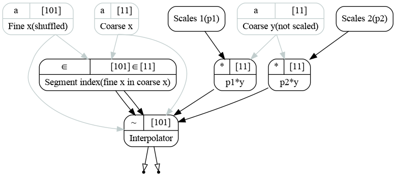
Calculation graph representing the interpolation process for two input functions.
Instead of using the automatic binding, one may bind the transformations manually as follows:
 1    # Bind transformations manually
 2    interpolator = R.InterpExpo(labels=labels)
 3
 4    edges  >> (interpolator.insegment.edges, interpolator.interp.x)
 5    points >> (interpolator.insegment.points, interpolator.interp.newx)
 6    interpolator.insegment.insegment >> interpolator.interp.insegment
 7    interpolator.insegment.widths    >> interpolator.interp.widths
 8    y1 >> interpolator.interp.y
 9    y2 >> interpolator.add_input()
10
11    interp1, interp2 = interpolator.interp.outputs.values()
Here we are using the syntax, explained earlier. We pass coarse \(x\) edges to the inputs of insegment and interp, then we do the same for fine \(z\) values (points). Then we pass outputs insegment and widths from the insegment to the interp. y1 is then binded to the first input while y2 is binded to the second input, created by add_input() method.
Two input functions may be interpolated by two distinct transformations within the same object. See the tutorial Lazy evaluation and graph structure for the more details on usage of add_input() and add_transformation() methods.
Now we leave all \(p_1\) values equal to 1 so the first graph represent the initial coarse function. For the second curve we set each odd parameter to 2 to compensate the saw-like structure.
1for par in list(pars2.values())[1::2]:
2    par.set(2.0)
After plotting y1 and y2 let us set each even \(p_1\) to 0.5 and plot again. The result may be found on the picture below.
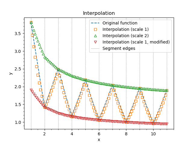
Example of exponential interpolation.
The dashed lines black represent the segment edges, the dashed blue line is the initial coarse function defined on these edges. Orange squares represent the interpolated function. They are slightly off the straight line since we have used exponential interpolation. Green triangles are for y2 and the red triangles are for y1 again after we scaled each even parameter down.
Note
There is InterpLinear object implementing linear interpolation. The syntax and transformations are similar to
ones from the InterpExpo.