8.1.4. 2d integration

8.1.4.1. Introduction

The formula for numerical 2d integration from Introduction

(1)\[\begin{split}H_{km} &= \int\limits_{a_k}^{a_{k+1}} dx \int\limits_{b_m}^{b_{m+1}} f(x, y)\,dy \approx \sum\limits_{i_k=1}^{K_k} \sum\limits_{j_m=1}^{M_m} \omega_{i_k}^x \omega_{j_m}^y f(x_{i_k}, y_{j_m}), \\ x_{i_k} &\in [a_i, a_{i+1}], \\ y_{j_m} &\in [b_j, b_{j+1}].\end{split}\]

implies that the function \(f(x,y)\) is computed on each pair of values of \(x\) and \(y\). Let’s write all the required values of \(x\) and \(y\) for all the bins as 1d arrays:

\[\begin{split}x = {x_1, x_2, \dotsc, x_N},\\ y = {y_1, y_2, \dotsc, x_M}.\end{split}\]

In order to have all the possible pairs we need to define two matrices (meshes) of size \(N\times M\). Values of \(x\) go over first dimension (rows) while values of \(y\) go to the second dimension (columns).

(2)\[\begin{split}&X_\text{mesh} = \begin{pmatrix} x_1 & x_1 & \dots & x_1 \\ x_2 & x_2 & \dots & x_2 \\ \vdots & \vdots & \ddots & \vdots \\ x_N & x_N & \dots & x_N \\ \end{pmatrix} \\ \\ &Y_\text{mesh} = \begin{pmatrix} y_1 & y_2 & \dots & y_M \\ y_1 & y_2 & \dots & y_M \\ \vdots & \vdots & \ddots & \vdots \\ y_1 & y_2 & \dots & y_M \\ \end{pmatrix}\end{split}\]

The value of the function is then computed as \(f_{ij}=f(X_\text{mesh}, Y_\text{mesh})\), on each pair of values. The output histogram is then defined as:

\[\begin{split}H_{km} \approx \sum\limits_{i\in k,\\j\in m} \omega_{ij} f_{ij}.\end{split}\]

8.1.4.2. 2d integral example

Let us now integrate the following function:

(3)\[f(x,y) = \sin(ax+by).\]

into 2d histograms with 20 bins over X axis \((-\pi,\pi)\) and 30 bins over Y axis \((0,2\pi)\). We choose constant integration orders: 4 points per bin for X and 3 points per bin for Y.

Just in case, its integral reads as follows:

\[\begin{split}&\int\limits_{x_1}^{x_2}dx \int\limits_{y_1}^{y_2}dy f(x,y) = \\ &= -\frac{1}{ab} \left( \sin( ax_2 + by_2 ) + \sin( ax_1 + by_1 ) - \sin( ax_2 + by_1 ) - \sin( ax_1 + by_2 ) \right).\end{split}\]

The procedure of performing the numerical integration is actually very similar to 1d case.

03_integral2d.py

import load
from gna.env import env
import gna.constructors as C
import numpy as np
from matplotlib import pyplot as plt
from gna.bindings import common
import ROOT as R
from mpl_toolkits.mplot3d import Axes3D

# Make a variable for global namespace
ns = env.globalns

# Create a parameter in the global namespace
pa = ns.defparameter('a', central=1.0, free=True, label='x scale')
pb = ns.defparameter('b', central=2.0, free=True, label='y scale')

# Print the list of parameters
ns.printparameters(labels=True)
print()

# Define binning and integration orders
x_nbins = 20
x_edges  = np.linspace(-np.pi, np.pi, x_nbins+1, dtype='d')
x_widths = x_edges[1:]-x_edges[:-1]
x_orders = 4

y_nbins = 30
y_edges  = np.linspace(0, 2.0*np.pi, y_nbins+1, dtype='d')
y_widths = y_edges[1:]-y_edges[:-1]
y_orders = 3

# Initialize histogram
hist = C.Histogram2d(x_edges, y_edges)

# Initialize integrator
integrator = R.Integrator2GL(x_nbins, x_orders, y_nbins, y_orders)
integrator.points.edges(hist.hist.hist)
int_points = integrator.points

# Create integrable: sin(a*x+b*y)
arg_t = C.WeightedSum( ['a', 'b'], [int_points.xmesh, int_points.ymesh] )
sin_t = R.Sin(arg_t.sum.sum)

# integrator.add_input(sint_t.sin.result)
integrator.hist.f(sin_t.sin.result)
X, Y = integrator.points.xmesh.data(), integrator.points.ymesh.data()

integrator.print()
print()

# Label transformations
hist.hist.setLabel('Input histogram\n(bins definition)')
integrator.points.setLabel('Sampler\n(Gauss-Legendre)')
integrator.hist.setLabel('Integrator\n(convolution)')
sin_t.sin.setLabel('sin(ax+by)')
arg_t.sum.setLabel('ax+by')

# Make 2d color plot
fig = plt.figure()
ax = plt.subplot(111, xlabel='x', ylabel='y', title=r'$\int\int\sin(ax+by)$')
ax.minorticks_on()
ax.set_aspect('equal')

# Draw the function and integrals
integrator.hist.hist.plot_pcolormesh(colorbar=True)

# Save figure
savefig(tutorial_image_name('png'))

# Add integration points and save
ax.scatter(X, Y, c='red', marker='.', s=0.2)
ax.set_xlim(-0.5, 0.5)
ax.set_ylim(0.0, 1.0)

savefig(tutorial_image_name('png', suffix='zoom'))

# Plot 3d function and a histogram
fig = plt.figure()
ax = plt.subplot(111, xlabel='x', ylabel='y', title=r'$\sin(ax+by)$', projection='3d')
ax.minorticks_on()
ax.view_init(elev=17., azim=-33)

# Draw the function and integrals
integrator.hist.hist.plot_surface(cmap='viridis', colorbar=True)
sin_t.sin.result.plot_wireframe_vs(X, Y, rstride=8, cstride=8)

# Save the figure and the graph
savefig(tutorial_image_name('png', suffix='3d'))
savegraph(sin_t.sin, tutorial_image_name('png', suffix='graph'), rankdir='TB')

plt.show()

The code produces the following graph. The sampler now produces two arrays for \(x\) and \(y\):, which are then passed to the computational chain representing the integrand function and the output of the chain is passed back to the integrator, which computes the histogram.

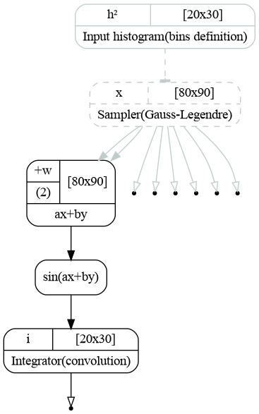
Computatinal graph used to compute double integral of a function \(f(x,y)=\sin(ax+by)\).

At first we create a 2d histogram to be used to define the bins:

hist = C.Histogram2d(x_edges, y_edges)

Then initialize 2d Gauss-Legendre integrator by providing number of bins and integration order(s) for each dimension and bind the histogram defining the bin edges.

integrator = R.Integrator2GL(x_nbins, x_orders, y_nbins, y_orders)
integrator.points.edges(hist.hist.hist)

An alternative way with bin edges passed as arguments reads as follows

integrator = R.Integrator2GL(x_nbins, x_orders, x_edges, y_nbins, y_orders, y_edges).

The status of the integrator object may be found below:

[obj] Integrator2GL: 2 transformation(s), 0 variables
     0 [trans] points: 1 input(s), 6 output(s)
         0 [in]  edges <- [out] hist: hist2d, 20x30=600 bins, edges -3.14159265359->3.14159265359 and 0.0->6.28318530718
         0 [out] x: array 1d, shape 80, size  80
         1 [out] y: array 1d, shape 90, size  90
         2 [out] xedges: array 1d, shape 21, size  21
         3 [out] yedges: array 1d, shape 31, size  31
         4 [out] xmesh: array 2d, shape 80x90, size 7200
         5 [out] ymesh: array 2d, shape 80x90, size 7200
     1 [trans] hist: 1 input(s), 1 output(s)
         0 [in]  f <- [out] result: array 2d, shape 80x90, size 7200
         0 [out] hist: hist2d, 20x30=600 bins, edges -3.14159265359->3.14159265359 and 0.0->6.28318530718

The transformation points contains 1d arrays with edges for X and Y axes (xedges and yedges), 1d arrays with integration points for X and Y axes (x and y). Finally it contains the 2d meshes (xmesh and ymesh) as defined in (2).

These meshes are then passed to the WeightedSum to be added with weights \(a\) and \(b\) and result of a sum is passed to the sine object.

arg_t = C.WeightedSum( ['a', 'b'], [int_points.xmesh, int_points.ymesh] )
sin_t = R.Sin(arg_t.sum.sum)

These two lines implement the function (3). The output of this function is passed to the integrator:

integrator.hist.f(sin_t.sin.result)

That is it. Then the output integrator.hist.hist contains the 2d histogram with integrated function, which may be plotted:

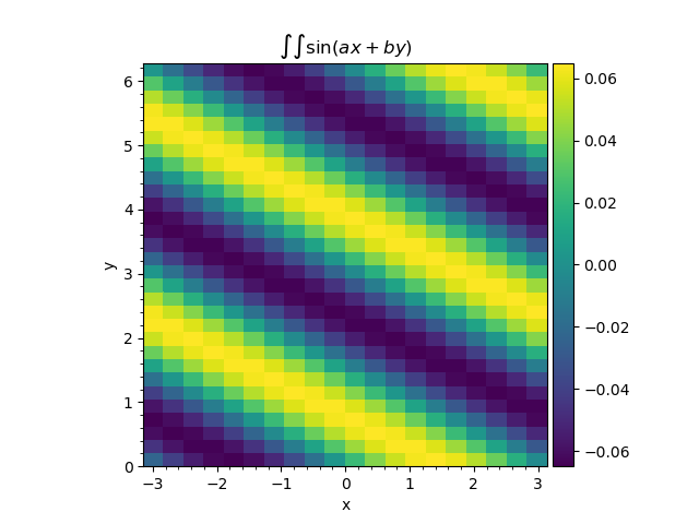
Double Gauss-Legendre quadrature application to the function (3).

We then zoom the plot to display the integration points.

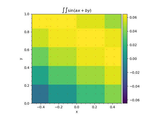
Double Gauss-Legendre quadrature application to the function (3). Red dots represent the integration points.

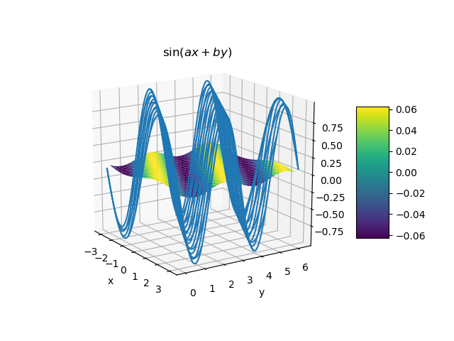
Double Gauss-Legendre quadrature application to the function (3) compared to the function itself.