8.1.3. More on 1d integration

Now let us repeat the previous study with several changes:

1. Try binning with variable widths as well as variable integration orders.

2. Check that changing variables affects the integration.

3. Use an alternative way of bin edges specification.

4. Use an alternative way of binding the function output.

5. Use an alternative integration method.

Here is the code:

02_integral1d_again.py

import load
from gna.env import env
import gna.constructors as C
import numpy as np
from matplotlib import pyplot as plt
import matplotlib.gridspec as gridspec
from gna.bindings import common
import ROOT as R

# Make a variable for global namespace
ns = env.globalns

# Create a parameter in the global namespace
pa = ns.defparameter('a', central=1.0, free=True, label='weight 1')
pb = ns.defparameter('b', central=0.2, free=True, label='weight 2')
pk = ns.defparameter('k', central=8.0, free=True, label='argument scale')

# Print the list of parameters
ns.printparameters(labels=True)
print()

# Define binning and integration orders
nbins = 20
x_edges = -np.pi + 2.0*np.pi*np.linspace(0.0, 1.0, nbins+1, dtype='d')**0.6
x_widths = x_edges[1:]-x_edges[:-1]
x_width_ratio = x_widths/x_widths.min()
orders = np.ceil(x_width_ratio*4).astype('i')

# Initialize histogram
hist = C.Histogram(x_edges)

# Initialize integrator
integrator = R.IntegratorTrap(nbins, orders)
integrator.points.edges(hist.hist.hist)
int_points = integrator.points.x

# Create integrable: a*sin(x) + b*cos(k*x)
cos_arg = C.WeightedSum( ['k'], [int_points] )
sin_t = R.Sin(int_points)
cos_t = R.Cos(cos_arg.sum.sum)
fcn   = C.WeightedSum(['a', 'b'], [sin_t.sin.result, cos_t.cos.result])

integrator.add_input(fcn.sum.sum)

integrator.print()
print()

# Label transformations
hist.hist.setLabel('Input histogram\n(bins definition)')
integrator.points.setLabel('Sampler\n(trapezoidal)')
integrator.hist.setLabel('Integrator\n(convolution)')
cos_arg.sum.setLabel('kx')
sin_t.sin.setLabel('sin(x)')
cos_t.cos.setLabel('cos(kx)')
fcn.sum.setLabel('a sin(x) + b cos(kx)')

# Compute the integral analytically as a cross check
# int| a*sin(x) + b*cos(k*x) = a*cos(x) - b/k*sin(kx) + C
a, b, k = (p.value() for p in (pa, pb, pk))
F = - a*np.cos(x_edges) + (b/k)*np.sin(k*x_edges)
integral_a = F[1:] - F[:-1]
bar_width = (x_edges[1:]-x_edges[:-1])*0.5
bar_left = x_edges[:-1]+bar_width

integral_n = integrator.hist.hist.data()

# Do some plotting
fig = plt.figure()
ax = plt.subplot(111)
ax.minorticks_on()
# ax.grid()
ax.set_ylabel( 'f(x)' )
ax.set_title(r'$a\,\sin(x)+b\,\sin(kx)$')

# Draw the function and integrals
fcn.sum.sum.plot_vs(int_points, 'o-', label='function at integration points', alpha=0.5, markerfacecolor='none', markersize=4.0)
integrator.hist.hist.plot_bar(label='integral: numerical', divide=2, shift=0, alpha=0.6)
ax.bar(bar_left, integral_a, bar_width, label='integral: analytical', align='edge', alpha=0.6)

# Freeze axis limits and draw bin edges
ax.autoscale(enable=True, axis='y')
ymin, ymax = ax.get_ylim()
ax.vlines(integrator.points.xedges.data(), ymin, ymax, linestyle='--', alpha=0.4, linewidth=0.5)

ax.legend(loc='lower right')

ymin, ymax = ax.get_ylim()

# Save figure and graph as images
savefig(tutorial_image_name('png', suffix='1'))

# Do more plotting
fig = plt.figure()
ax = plt.subplot(111)
ax.minorticks_on()
# ax.grid()
ax.set_ylabel( 'f(x)' )
ax.set_title(r'$a\,\sin(x)+b\,\sin(kx)$')
ax.autoscale(enable=True, axis='y')
ax.set_ylim(ymin, ymax)
ax.axhline(0.0, linestyle='--', color='black', linewidth=1.0, alpha=0.5)

def plot_sample():
    label = 'a={}, b={}, k={}'.format(*(p.value() for p in (pa,pb,pk)))
    lines = fcn.sum.sum.plot_vs(int_points, '--', alpha=0.5, linewidth=1.0)
    color = lines[0].get_color()
    integrator.hist.hist.plot_hist(alpha=0.6, color=color, label=label)

plot_sample()
pa.set(-0.5)
pk.set(16)
plot_sample()
pa.set(0)
pb.set(0.1)
plot_sample()

# Freeze axis limits and draw bin edges
ymin, ymax = ax.get_ylim()
ax.vlines(integrator.points.xedges.data(), ymin, ymax, linestyle='--', alpha=0.4, linewidth=0.5)
ax.legend(loc='lower right')

plt.show()

First of all, instead of passing the bin edges as an argument we make a histogram first.

hist = C.Histogram(x_edges)

Usually we would like to have only one bins definition for the computational chain, thus, if several integrations occur, it is more convenient to provide bin edges via input.

integrator = R.IntegratorTrap(nbins, orders)
integrator.points.edges(hist.hist.hist)

Note that the integrator is created without bins passed as an argument. Only in this case the points.edges input is created. The variable orders now contains a numpy array with integers. Instead of Gauss-Legendre in this example we will use the trapezoidal integration.

Then we use the similar function as we have used in the previous example. Instead of binding it directly we use a method add_input(output). This method may be used several times. On each execution it will create and bind a new input. A new output is created for each input. Thus for the same bins and orders the transformation may calculate several integrals within one execution.

integrator.add_input(fcn.sum.sum)

The method returns the corresponding output.

Note, that because of the taintflag propagation, even in case only one input is tainted, all the integrals will be recalculated. Multiple transformations should be used in case such a behaviour is not desired.

The code produces the following computational chain:

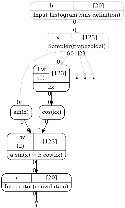
Computatinal graph used to integrate function \(f(x)=a\sin(x)+b\cos(kx)\). The bin edges are passed via input.

Then we repeat the same procedure with cross checking the calculation. The plot below illustrates the variable bin widths as well as variable integration orders.

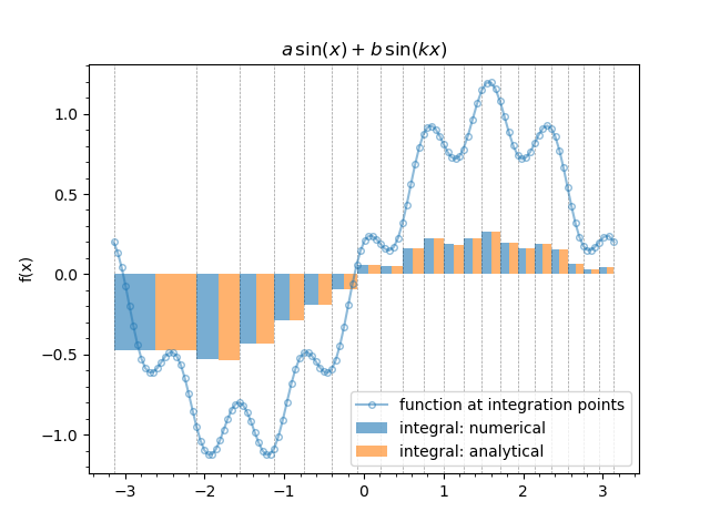
The trapezoidal quadrature application to the function (1). Variable bin width and different integration orders per bin.

In order to illustrate the impact of the parameters on the results let us create a function, that plots function (1), its integrals for the current values of the parameters:

def plot_sample():
    label = 'a={}, b={}, k={}'.format(*(p.value() for p in (pa,pb,pk)))
    lines = fcn.sum.sum.plot_vs(int_points, '--', alpha=0.5, linewidth=1.0)
    color = lines[0].get_color()
    integrator.hist.hist.plot_hist(alpha=0.6, color=color, label=label)

Now we make three plots for different values of the parameters:

plot_sample()
pa.set(-0.5)
pk.set(16)
plot_sample()
pa.set(0)
pb.set(0.1)
plot_sample()

The result is shown on the figure below:

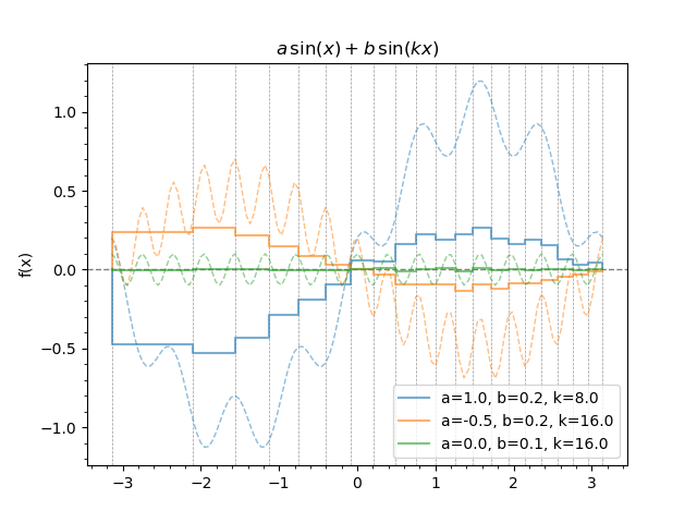
The trapezoidal quadrature application to the function (1) for different values of the parameters \(a\), \(b\) and \(k\).