11.1. Fitting to Asimov dataset
Let us now construct an example setup for fitting. We will use gaussianpeak module to provide both the data and the model to be fit.
At first, we initialize two gaussianpeak modules with names peak_MC and peak_f. The former will be used as data while the latter will be used as a model to be fit.
1./gna \
2      -- gaussianpeak --name peak_MC --nbins 50 \
3      -- gaussianpeak --name peak_f  --nbins 50 \
Now, using ns module we change the parameters for the models:
 1      -- ns --name peak_MC --print \
 2            --set E0             values=2    fixed \
 3            --set Width          values=0.5  fixed \
 4            --set Mu             values=2000 fixed \
 5            --set BackgroundRate values=1000 fixed \
 6      -- ns --name peak_f --print \
 7            --set E0             values=2    free \
 8            --set Width          values=0.5  free \
 9            --set Mu             values=2000 free \
10            --set BackgroundRate values=1000 free \
Here we have used slightly different approach to the parameters. Instead of defining the parameters prior the models, we
change them after the module creates the default versions. Syntax of the --set option is pretty similar to the
one of the --define.
This command line produces the following output:
 1Add observable: peak_MC/spectrum
 2Add observable: peak_f/spectrum
 3Variables in namespace 'peak_MC':
 4  BackgroundRate                =       1000 │                 [fixed]                 │ Flat background rate 0
 5  Mu                            =       2000 │                 [fixed]                 │ Peak 0 amplitude
 6  E0                            =          2 │                 [fixed]                 │ Peak 0 position
 7  Width                         =        0.5 │                 [fixed]                 │ Peak 0 width
 8Variables in namespace 'peak_f':
 9  BackgroundRate                =       1000 │        1000±           5 [free]         │ Flat background rate 0
10  Mu                            =       2000 │        2000±          10 [free]         │ Peak 0 amplitude
11  E0                            =          2 │           2±        0.05 [free]         │ Peak 0 position
12  Width                         =        0.5 │         0.5±       0.005 [free]         │ Peak 0 width
Next step is to define the Datasets and Analysis instances. Both of them should have unique name defined. Names should be unique across the similar modules: all datasets should have unique names and all analysis should have unique names, there still may exist a dataset and an analysis with the same name.
The Dataset is defined by the dataset module.
-- dataset --name peak --asimov-data peak_f/spectrum peak_MC/spectrum \
We have just created dataset peak, that makes a correspondence between the output peak_f/spectrum and output
peak_MC/spectrum (data). The option --asimov-data indicates that peak_MC will have no fluctuations added.
In addition to data and theory outputs dataset defines statistical uncertainties. They are optional in a sense, that they may be used by the static, for example by \(\chi^2\) function. In case log-Poisson is used the statistical uncertainties defined in data set will be ignored.
Attention
By default Pearson’s definition for statistical uncertainties is used: For each bin \(i\) \(\sigma_\text{stat}=\sqrt{N_i}\), where \(N_i\) comes from theory. Therefore statistical uncertainties depend on the actual parameter values used for the theory at the current step.
Statistical uncertainties output is frozen and will not be updated when minimizer will change the parameters.
In case of a single Asimov dataset the Analysis definition is straightforward:
-- analysis --name analysis --datasets peak \
Here we define Analysis, named analysis, which is using a single dataset peak. The analysis now may be used to define the statistics. Let us use the \(\chi^2\) statistics:
-- chi2 stats_chi2 analysis \
The syntax is similar. The module chi2 defines the \(\chi^2\) statistics with name stats_chi2 and assigns it to the analysis analysis.
In order to create the minimizer one needs to define its name, type, statistics and a set of parameters to minimize. Parameters may be defined either as a list of parameter names or the namespace names. All the parameters from the namespaces, mentioned in the command, will be used for minimization.
-- minimizer min minuit stats_chi2 peak_f \
Here we define the minimizer min, which will use ROOT’s Minuit to minimize the statistics stats_chi2, which depends on the parameters, listed in the namespace peak_f.
For the illustration purpose let us now change the parameters for the minimization:
      -- ns --name peak_f --print \
            --set E0             value=3    \
            --set Width          value=0.2  \
            --set Mu             value=100  \
            --set BackgroundRate value=2000 \
Now we may plot the data and initial state of the model with the following command line:
      -- spectrum -p peak_MC/spectrum -l 'Monte-Carlo' --plot-type errorbar \
      -- spectrum -p peak_f/spectrum -l 'Model (initial)' \
      -- mpl-v1 --xlabel 'Energy, MeV' --ylabel entries --grid -s \
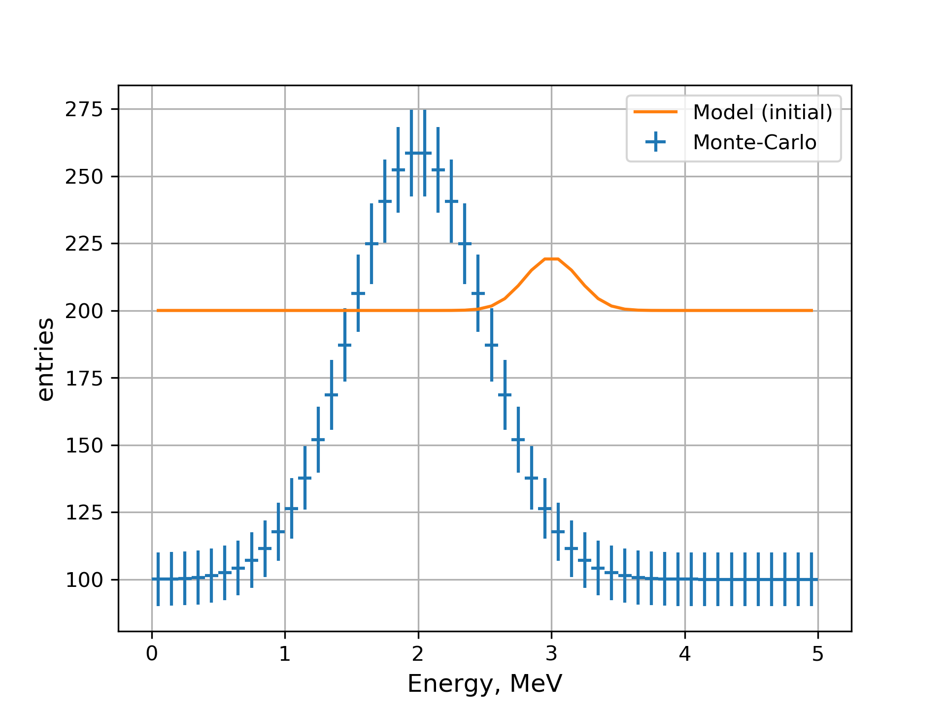
MC data defined by the model peak_MC and initial state of the model peak_f.
The minimizer module only creates minimizer, but does not use it for the minimization. It may then be used from other modules to find a best fit, estimate confidence intervals, etc. The fitting may be invoked from the fit module:
-- fit min -s -p -o output/fit_01.yaml \
This simple module performs a fit, prints the result to standard output (-p option) and saves it to the output
file (-o option). After the minimization is done, the best fit values, estimated uncertainties, function at the
minimum are printed as well as some usage statistics.
 1Fit result:${
 2  cpu : 0.027739163997466676,
 3  errors : [21.044786843888083, 89.87411551001028, 0.019925689550693886, 0.021573688772678953],
 4  errorsdict : ${
 5    peak_f : ${
 6      BackgroundRate : 21.044786843888083,
 7      E0 : 0.019925689550693886,
 8      Mu : 89.87411551001028,
 9      Width : 0.021573688772678953,
10    },
11  },
12  fun : 4.6533546220329065e-08,
13  maxcv : 0.01,
14  names : ['peak_f.BackgroundRate', 'peak_f.Mu', 'peak_f.E0', 'peak_f.Width'],
15  nfev : 166,
16  npars : 4,
17  success : True,
18  wall : 0.02774786949157715,
19  x : [1000.000584000211, 1999.989446718792, 2.0000031405938894, 0.4999998136336317],
20  xdict : ${
21    peak_f : ${
22      BackgroundRate : 1000.000584000211,
23      E0 : 2.0000031405938894,
24      Mu : 1999.989446718792,
25      Width : 0.4999998136336317,
26    },
27  },
28}
The minimizer takes care so that original values of the parameters were restored after the minimization process.
Extra option -s/--set makes fitter to set the best fit values to the model, unless the fit failed.
Now we can plot the state of the fit model.
      -- mpl --figure \
      -- spectrum -p peak_MC/spectrum -l 'Monte-Carlo' --plot-type errorbar \
      -- spectrum -p peak_f/spectrum -l 'Best fit model' \
      -- mpl --xlabel 'Energy, MeV' --ylabel entries --grid \
             -o output/fit_01.pdf -s
The ns module prints the current and default values of the parameters to the output:
Save output file: output/tutorial_img/fit/01_fit_models.yaml
Variables in namespace 'peak_f':
  BackgroundRate                =       1000 │        1000±           5 [free]         │ Flat background rate 0
  Mu                            =    1999.99 │        2000±          10 [free]         │ Peak 0 amplitude
  E0                            =          2 │           2±        0.05 [free]         │ Peak 0 position
The result of the fitting is:
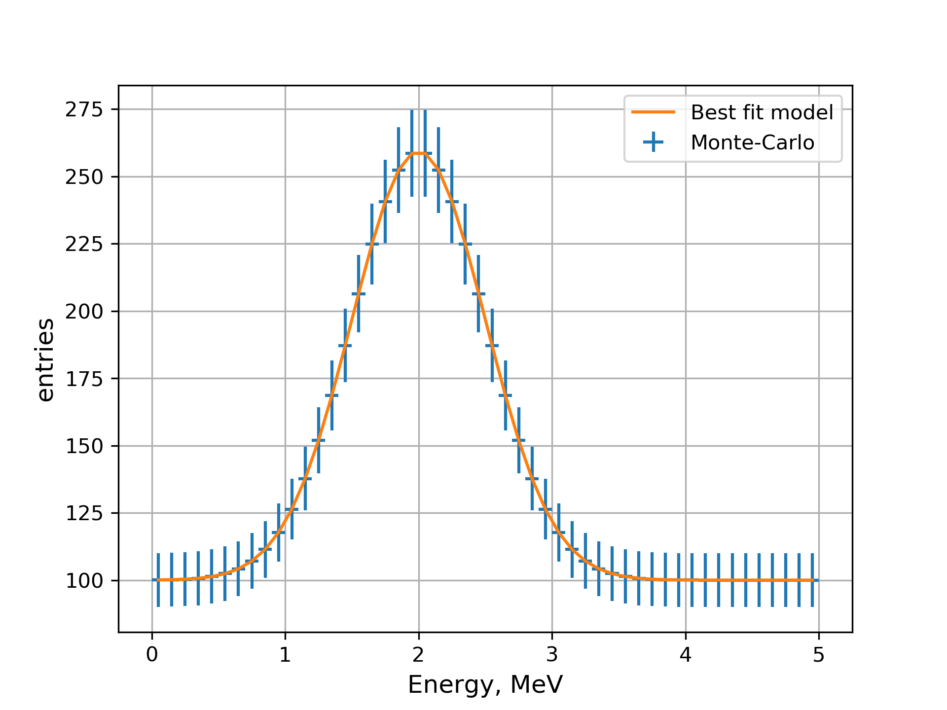
MC data defined by the model peak_MC and best fit state of the model peak_f.
As soon as the model contains no fluctuations, the function at the minimum is consistent with zero: \(\chi^2_\text{min}\lesssim10^{-8}\).
Also, the fit module have saved readable version of the result to the file fit_01.yaml in the YAML format, which can be later loaded back into python.
The full version of the command is below:
 1#!/bin/bash
 2
 3./gna \
 4      -- gaussianpeak --name peak_MC --nbins 50 \
 5      -- gaussianpeak --name peak_f  --nbins 50 \
 6      -- ns --name peak_MC --print \
 7            --set E0             values=2    fixed \
 8            --set Width          values=0.5  fixed \
 9            --set Mu             values=2000 fixed \
10            --set BackgroundRate values=1000 fixed \
11      -- ns --name peak_f --print \
12            --set E0             values=2    free \
13            --set Width          values=0.5  free \
14            --set Mu             values=2000 free \
15            --set BackgroundRate values=1000 free \
16      -- dataset  --name peak --asimov-data peak_f/spectrum peak_MC/spectrum \
17      -- analysis --name analysis --datasets peak \
18      -- graphviz peak_f/spectrum -o output/fit_01_graph.pdf \
19      -- chi2 stats_chi2 analysis \
20      -- ns --name peak_f --print \
21            --set E0             value=3    \
22            --set Width          value=0.2  \
23            --set Mu             value=100  \
24            --set BackgroundRate value=2000 \
25      -- minimizer min minuit stats_chi2 peak_f \
26      -- spectrum -p peak_MC/spectrum -l 'Monte-Carlo' --plot-type errorbar \
27      -- spectrum -p peak_f/spectrum -l 'Model (initial)' \
28      -- mpl-v1 --xlabel 'Energy, MeV' --ylabel entries --grid -s \
29      -- fit min -s -p -o output/fit_01.yaml \
30      -- ns --print peak_f \
31      -- mpl --figure \
32      -- spectrum -p peak_MC/spectrum -l 'Monte-Carlo' --plot-type errorbar \
33      -- spectrum -p peak_f/spectrum -l 'Best fit model' \
34      -- mpl --xlabel 'Energy, MeV' --ylabel entries --grid \
35             -o output/fit_01.pdf -s
11.1.1. Saving fit result to other formats
The result may be saved to the pickle binary format. In order to achieve this the output extension should be set to .pkl:
... \
-- fit min -s -p -o output/fit_01.pkl \
... \
The -o option accepts multiple arguments, so the output may be saved into multiple files:
... \
-- fit min -s -p -o output/fit_01.pkl output/fit_01.yaml \
... \
While YAML is easier to read, the pickle binary format loads faster.