4.2. Plotting outputs in 2d: 2d histograms

4.2.1. Matrices

The plot_matshow(...) method is defined implementing matshow(A, …) call passing output contents as A. This method works with both histograms and arrays. When applied to histograms it ignores bin edges definitions and plots the matrix anyway: first dimension defines rows, second - columns; the rows are plotted over Y axis and columns of X axis.

03_matshow.py

import gna.constructors as C
import numpy as np
from gna.bindings import common

# Create numpy arrays for 1d and 2d cases
narray2 = np.arange(20).reshape(5,4)
# Create a Points instance
parray2 = C.Points(narray2)

print('Data 2d:\n', parray2.points.points.data())

from matplotlib import pyplot as plt
fig = plt.figure()
ax = plt.subplot( 111 )
ax.minorticks_on()
ax.set_xlabel( 'x label' )
ax.set_ylabel( 'y label' )
ax.set_title( 'Plot title' )

parray2.points.points.plot_matshow(mask=0.0, colorbar=True)

plt.show()

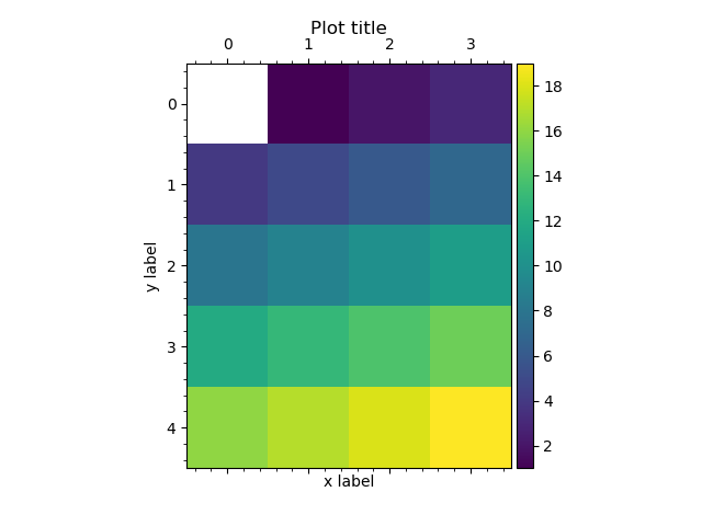
An example output2d.plot_matshow() method for outputs.

Keyword options

colorbar=True	add a colorbar
colorbar=dict(…)	add a colorbar and pass the options to colorbar()
mask	do not colorize values, equal to mask. mask=0.0 will produce ROOT-like colormaps
transpose=True	transpose arrays before plotting

Note

Unlike in matplotlib output.matshow() will not create extra figure by default. See fignum option description in matshow() documentation.

4.2.2. 2d histograms with constant binning

There are several options to plot 2d histograms as histograms, i.e. with first dimension over X and second dimension over Y. In case the histogram has bins of equal width plot_pcolorfast() or plot_imshow() may be used. Both methods support the same extra options as matshow.

4.2.2.1. pcolorfast

plot_pcolorfast(...) method implements a pcolorfast(X, Y, C, …) call passing output contents as X, Y and C. Below see an example of Gaussian with width 10 for X and width 3 for Y.

06_hist2d_plot_equal.py

import gna.constructors as C
import numpy as np
from gna.bindings import common
from matplotlib import pyplot as plt
# Create numpy array for data points
xmin, ymin = 10, 20
nbinsx, nbinsy = 40, 50
edgesx = np.linspace(xmin, xmin+nbinsx*0.5, nbinsx+1)
edgesy = np.linspace(ymin, ymin+nbinsy*0.5, nbinsy+1)
# Create fake data array
cx = (edgesx[1:] + edgesx[:-1])*0.5
cy = (edgesy[1:] + edgesy[:-1])*0.5
X, Y = np.meshgrid(cx, cy, indexing='ij')
narray = np.exp(-0.5*(X-15.0)**2/10.0**2 - 0.5*(Y-30.0)**2/3.0**2)

# Create a histogram instance with data, stored in `narray`
# and edges, stored in `edges`
hist = C.Histogram2d(edgesx, edgesy, narray)

fig = plt.figure()
ax = plt.subplot( 111 )
ax.set_title( 'pcolorfast' )
ax.minorticks_on()
ax.set_xlabel( 'x label' )
ax.set_ylabel( 'y label' )

hist.hist.hist.plot_pcolorfast(colorbar=True)

plt.show()

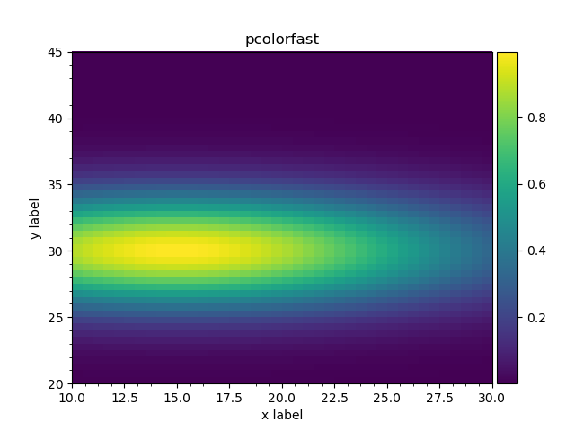
2d histogram plotted via plot_pcolorfast() method.

4.2.2.2. imshow

The second method plot_imshow() is using imshow(X, …) passing output data as X. The imshow() method is designed to show images and thus it sets the equal visual size for x and y intervals [1].

06_hist2d_plot_equal.py

hist.hist.hist.plot_imshow(colorbar=True)

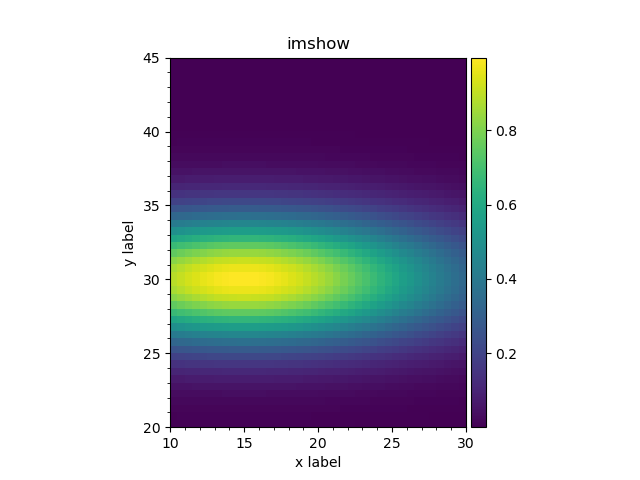
2d histogram plotted via plot_imshow() method.

[1]

Similar effect may be achieved to any plot with ax.set_aspect('equal').

4.2.2.3. matshow

The relevant plot produced by the plot_matshow() may be found below.

06_hist2d_plot_equal.py

hist.hist.hist.plot_matshow(colorbar=True)

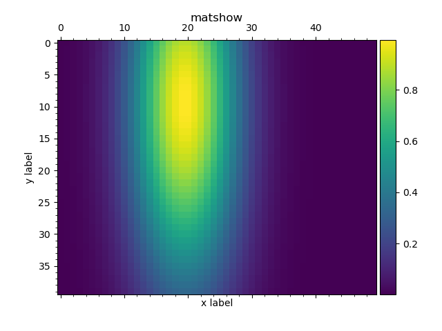
2d histogram, plotted as matrix.

4.2.3. 2d histograms with variable binning

In case histograms have bins of variable size plot_pcolormesh() method should be used. It is using pcolormesh(X, Y, C, …) call passing output data as X, Y and C. The method essentially works for the constant binning histograms as well. The method supports the same extra options as matshow.

We will use a Gaussian with width 150 for X and 0.1 for Y.

06_hist2d_plot.py

import gna.constructors as C
import numpy as np
from gna.bindings import common
from matplotlib import pyplot as plt
# Create numpy array for data points
xmin, ymin = 10, 20
nbinsx, nbinsy = 40, 50
edgesx = np.linspace(xmin, xmin+nbinsx*0.5, nbinsx+1)**2
edgesy = np.linspace(ymin, ymin+nbinsy*0.5, nbinsy+1)**0.25
# Create fake data array
cx = (edgesx[1:] + edgesx[:-1])*0.5
cy = (edgesy[1:] + edgesy[:-1])*0.5
X, Y = np.meshgrid(cx, cy, indexing='ij')
narray = np.exp(-0.5*(X-cx[15])**2/150.0**2 - 0.5*(Y-cy[20])**2/0.10**2)

# Create a histogram instance with data, stored in `narray`
# and edges, stored in `edges`
hist = C.Histogram2d(edgesx, edgesy, narray)

fig = plt.figure()
ax = plt.subplot( 111 )
ax.set_title( 'pcolormesh' )
ax.minorticks_on()
ax.set_xlabel( 'x label' )
ax.set_ylabel( 'y label' )

hist.hist.hist.plot_pcolormesh(colorbar=True)

plt.show()

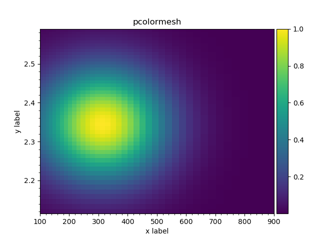
2d histogram with variable binning.

In addition, the method plot_pcolor() can be used.