10.2. Example: initializing and plotting a model

10.2.1. Creating and plotting a model

Let us now use gaussianpeak module to create a simple module with integrated Gaussian function. The command

./gna -- \
      -- gaussianpeak --name peak

Creates a computational chain with integration and registers the output in the environment as peak/spectrum. This is registered in the output as:

Add observable: peak/spectrum

This output now may be used from the other modules. For example, we may plot it with plot-spectrum module.

We will use multi-line commands for better readability. Note, that \ at the end of each line should have no spaces afterwards.

./gna -- \
      -- gaussianpeak --name peak \
      -- plot-spectrum -p peak/spectrum \
      -- mpl -s

The module plot-spectrum adds the output to the figure after -p <name> option. Argument -s enables plot-spectrum to show the window with plotted figure after execution. The command will produce the following plot.

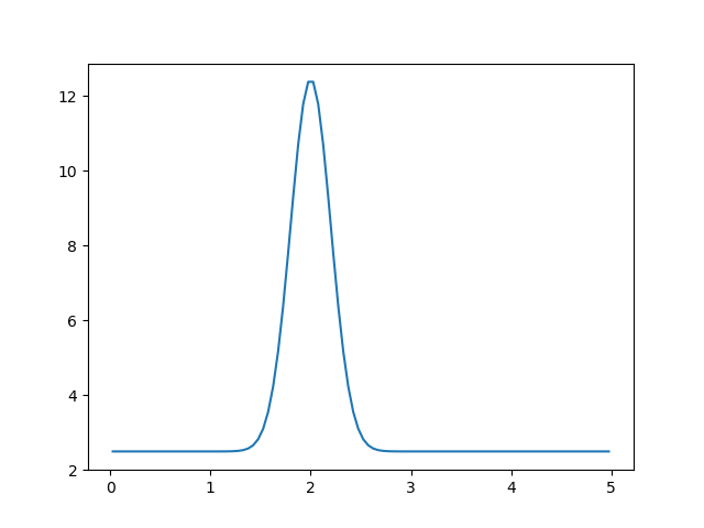
The spectrum, created by the gaussianpeak module and plotted via plot-spectrum module.

Both modules have options, that enable us to control the parameters. Let us define the energy range and number of bins (see ./gna – gaussianpeak –help for reference). Also let us define the figure title and axes labels (see ./gna – plot-spectrum –help for reference):

./gna -- \
      -- gaussianpeak --name peak --Emin 0 --Emax 5 --nbins 200 \
      -- plot-spectrum -p peak/spectrum -l 'Peak 1' \
      -- mpl -t 'Gaussian Peak' --xlabel 'Energy, MeV' --ylabel '$dN/dE$' -s

The modified command produces now annotated plot:

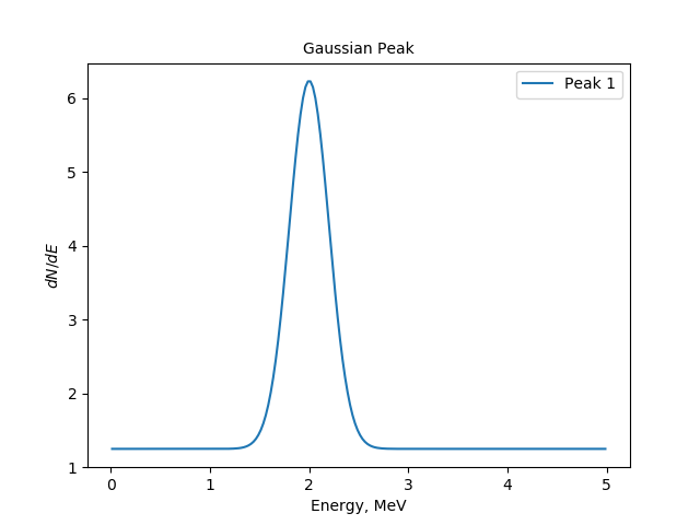
The spectrum, created by the gaussianpeak module and plotted via plot-spectrum module.

Finally, let us save the image using -o <filename.pdf> option. With use --latex command to enable matplotlib use latex for better rendering.

Also let us save the graph of the example model. The graphviz module reads the output name as the first argument.

./gna -- \
      -- gaussianpeak --name peak --Emin 0 --Emax 5 --nbins 200 --print \
      -- graphviz peak/spectrum -o output/gna_ui_graph.pdf \
      -- plot_spectrum -p peak/spectrum -l 'Peak 1' \
      -- mpl --ylim 0.0 -t 'Gaussian Peak' \
             --xlabel 'Energy, MeV' --ylabel '$dN/dE$' \
             -s --latex -o output/gna_ui_figure.pdf

The model is represented by the following graph:

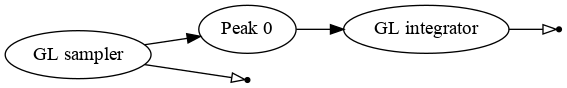
The computational chain created by the gaussianpeak module.

The chain consists of a single GuaissianPeak transformation, implementing a sum of a normal distribution and flat background. The function is integrated with Gauss-Legendre integrator.

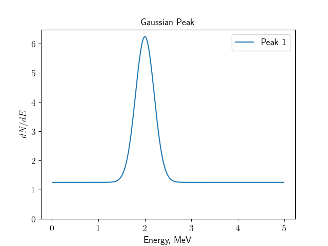
The spectrum, created by the gaussianpeak module.

Note

Do not forget to create output folder.

10.2.2. Changing the parameter values

Remember, that parameters are not owned neither by transformations, nor by the modules the transformations are created in. The parameters are usually initialized with reqparameter() command which only creates anything when no parameters with the same name was defined before.

The module gaussianpeak also prints a list of the variables it creates, when argument --print is passed:

Variables in namespace 'peak':
BackgroundRate       =         50 │          50±           5 [         10%] │ Flat background rate 0
Mu                   =        100 │         100±          10 [         10%] │ Peak 0 amplitude
E0                   =          2 │           2±        0.05 [        2.5%] │ Peak 0 position
Width                =        0.2 │         0.2±       0.005 [        2.5%] │ Peak 0 width

They are the contribution of the flat background and the parameters of the peak: position, width and amplitude, defined as follows:

\[\frac{d N}{d E} = b + \mu \frac{1}{\sqrt{2\pi w}}\exp{\frac{-(E-E_0)^2}{2w^2}}\]

All of these parameters may be overridden from the command line via ns module. As usual the help may be requested via

./gna -- ns --help command. Main ns commands include:

./gna -- ns --print \
    --define var1    central=1 fixed=True label='Fixed variable' \
    --define var2    central=2 sigma=0.5  label='Constrained variable' \
    --define ns.var3 central=3 free=True label='Free nested variable'

The syntax is similar to that described in tutorial on parameters. The :code:--print argument makes ns print the global namespace.

Variables in namespace '':
  var1                 =          1 │                 [fixed]                 │ Fixed variable
  var2                 =          2 │           2±         0.5 [         25%] │ Constrained variable
Variables in namespace 'ns':
  var3                 =          3 │           3±         inf [free]         │ Free nested variable

A namespace name may follow the --print argument. Thus --print ns will print only the last parameter.

Now by using ns module we may tune the parameters for the gaussianpeak model. As one may see from the printout above, the gaussianpeak parameters are defined in the namespace peak. Therefore, we may predefine them.

The following command line lower the background rate twice, moves the peak position to 6 (MeV) and changes its width to 2 MeV. We also increase the range to 12 MeV as well as the number of bins.

./gna -- ns \
            --define peak.BackgroundRate central=25  fixed=True label='Background rate' \
            --define peak.E0             central=6   fixed=True label='Peak position' \
            --define peak.Width          central=2   fixed=True label='Peak width' \
      -- gaussianpeak --name peak --Emin 0 --Emax 12 --nbins 480 --print \
      -- plot_spectrum -p peak/spectrum -l 'Peak 1' \
      -- mpl --ylim 0.0 -t 'Gaussian Peak' \
             --xlabel 'Energy, MeV' --ylabel '$dN/dE$' \
             -s

The command produces the following plot:

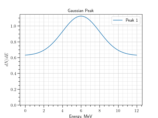
The spectrum, created by the gaussianpeak module with modified parameters.